PySINDy SCiML workshop

Installing PySINDy

To install the newest version of PySINDy, you must follow the instructions on the documentation. The version available through Conda is much older than the newest release. See https://pysindy.readthedocs.io/en/latest/index.html#installation.

!pip install pysindy --quiet

[2K     [90m━━━━━━━━━━━━━━━━━━━━━━━━━━━━━━━━━━━━━━━━[0m [32m121.0/121.0 kB[0m [31m3.1 MB/s[0m eta [36m0:00:00[0m
[?25h

import matplotlib.pyplot as plt
from mpl_toolkits.mplot3d import Axes3D
import numpy as np
from scipy.integrate import solve_ivp
from sklearn.metrics import mean_squared_error

import os
#print(os.getcwd())
#os.chdir("../PhD/PhD/ANAET")
from pysindy.utils import lorenz, lorenz_control, enzyme
import pysindy as ps

# bad code but allows us to ignore warnings
import warnings
from scipy.integrate.odepack import ODEintWarning
warnings.simplefilter("ignore", category=UserWarning)
warnings.simplefilter("ignore", category=FutureWarning)
warnings.simplefilter("ignore", category=ODEintWarning)

# Seed the random number generators for reproducibility
np.random.seed(100)

# Initialize integrator keywords for solve_ivp to replicate the odeint defaults
integrator_keywords = {}
integrator_keywords['rtol'] = 1e-12
integrator_keywords['method'] = 'LSODA'
integrator_keywords['atol'] = 1e-12

import matplotlib as mpl
mpl.rcParams["xtick.labelsize"]=22
mpl.rcParams["ytick.labelsize"]=22
mpl.rcParams["axes.labelsize"]=26
mpl.rcParams['mathtext.fontset'] = 'stix'
mpl.rcParams['font.family'] = 'STIXGeneral'

<ipython-input-3-92171691bfc6>:15: DeprecationWarning: Please use `ODEintWarning` from the `scipy.integrate` namespace, the `scipy.integrate.odepack` namespace is deprecated.
  from scipy.integrate.odepack import ODEintWarning

Starting with PySINDy

In this section, we start by using the Lorenz system for identification. The equations have the form \begin{align} \dot{x} & = \sigma (y-x),
\dot{y} & = x(\rho-z) -y,
\dot{z} & = xy - \beta z \end{align} where $\sigma, \rho, \beta$ are scalars. The first example shows how pySINDy can be used to reproduce the results of the original paper (Brunton et al 2016).

Tasks

Run the example script below, try changing the different fitting parameters. Change the time-stepping in the training data. How does this impact the model fit?
Vary the library size and calculate the error on the test trajectory, how can you use this to select the library?
Train the lorenz equations with the parameters $(10, 8/3, 6)$ with an initial condition $[-3.65, -3.65, 5]$. Why does model identification fail for this case?
Now train the Lorenz model with the same parameters, but using the initial condition $[-8, 8, 27]$ between $t \in [0, 0.5]$ for a time-step of $dt = 0.0001$. Can you successfully identify the correct equations using a second order polynomial library?
Now parameterise the Lorenz model through the bifurcation in the parameter $\rho$

# define the testing and training Lorenz data we will use for these examples
dt = 0.001
integrator_keywords["args"] = (10, 8/3, 28)

## create a training set of data
t_train = np.arange(0, 10, dt)
x0_train = [-8, 8, 27]
t_train_span = (t_train[0], t_train[-1])
x_train = solve_ivp(
    lorenz, t_train_span, x0_train, t_eval=t_train, **integrator_keywords
).y.T

## create a test set of data
t_test = np.arange(0, 15, dt)
t_test_span = (t_test[0], t_test[-1])
x0_test = np.array([8, 7, 15])
x_test = solve_ivp(
    lorenz, t_test_span, x0_test, t_eval=t_test, **integrator_keywords
).y.T


feature_names = ['x', 'y', 'z']
#define a library
feature_library = ps.PolynomialLibrary(5)
sparse_regression_optimizer = ps.STLSQ(threshold=0.01, alpha =0.01)  # default is lambda = 0.1
model = ps.SINDy(feature_names=feature_names,
                 feature_library = feature_library,
                 optimizer=sparse_regression_optimizer)
model.fit(x_train, t=t_train)
model.print(precision=4)

prediction = model.simulate(x_test[0,:], t_test)

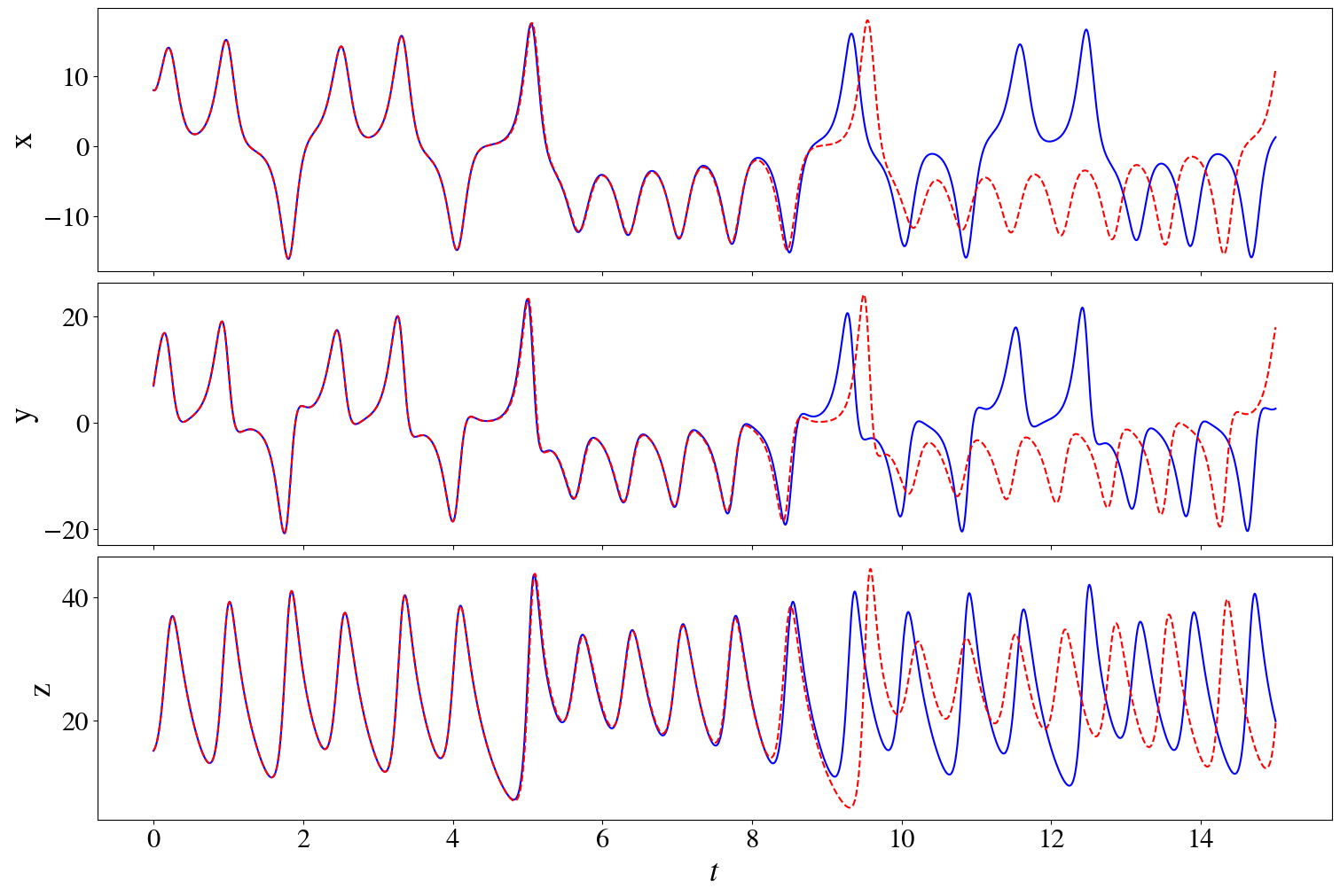
#plot the prediction against the test data
fig, ax = plt.subplots(3,1, figsize=(15,10), sharex=True, layout="constrained")
for i in range(3):
    ax[i].plot(t_test, x_test[:,i], "b")
    ax[i].plot(t_test, prediction[:,i], "--r")
    ax[i].set_ylabel(feature_names[i])
ax[-1].set_xlabel(r"$t$")

print("mean squared error on test data", model.score(x_test, t=t_test, metric=mean_squared_error))

(x)' = -9.9998 x + 9.9998 y
(y)' = 27.9980 x + -0.9996 y + -0.9999 x z
(z)' = -2.6666 z + 1.0000 x y
mean squared error on test data 4.619382264489079e-06

png

Mean field model

One reduced-order model of flow past a cylinder is the coupled system of equations \begin{align} \dot{x} &= \mu x- \omega y - xz,
\dot{y} &= \mu y + \omega x -yz,
\dot{z} & = -z + x^2 + y^2 \end{align} where $\mu$ and $\omega$ are scalars. $\omega$ gives the frequency of oscillation.

Tasks:

Generate a training set of data using the initial conditions $[0.01, 0.01, 0.1]$, $\omega=1$ and $\mu=0.1$. Use SINDy to identify the model.
Now fit a SINDy model to data only when the model is on the stable limit cycle (the data is only oscillating). What happens to the model?

mu = 0.1
omega =1
A=-1
lam = 1
def cylinder_wake(t, xv):
    x,y,z = xv
    return [mu*x-omega*y+A*x*z,
            omega*x + mu*y + A*y*z,
            -z+x**2+y**2]
y0 = [0.01, 0.01, 0.1]

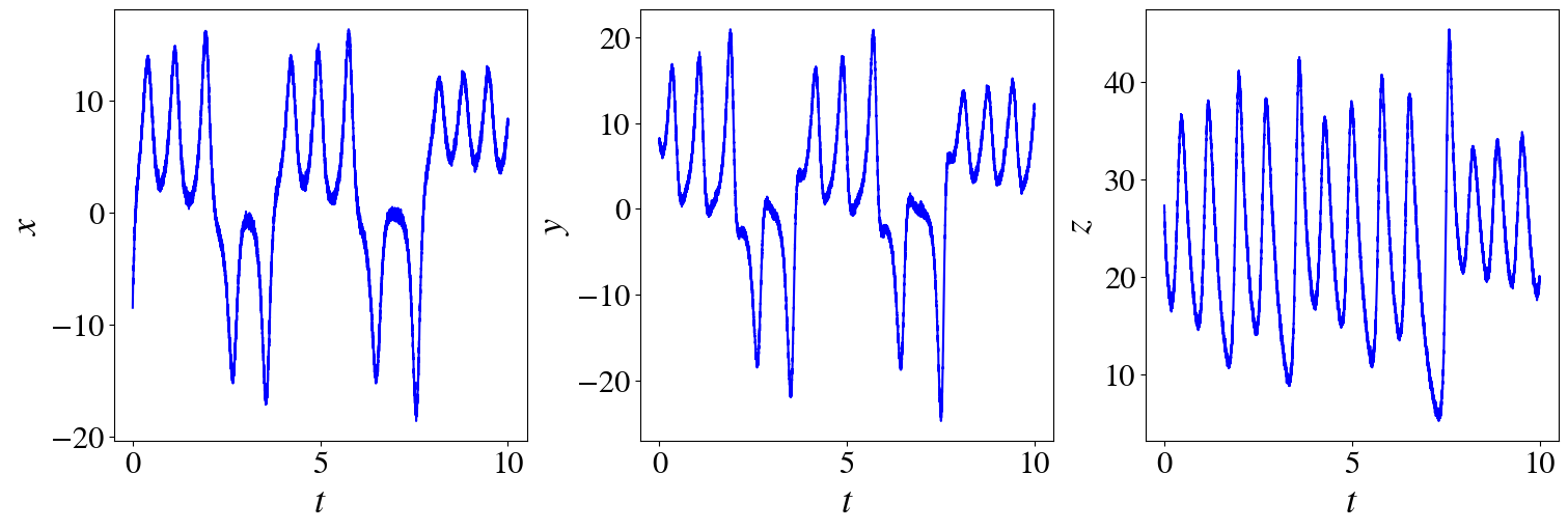
Coding challenge, identifying a model with noise

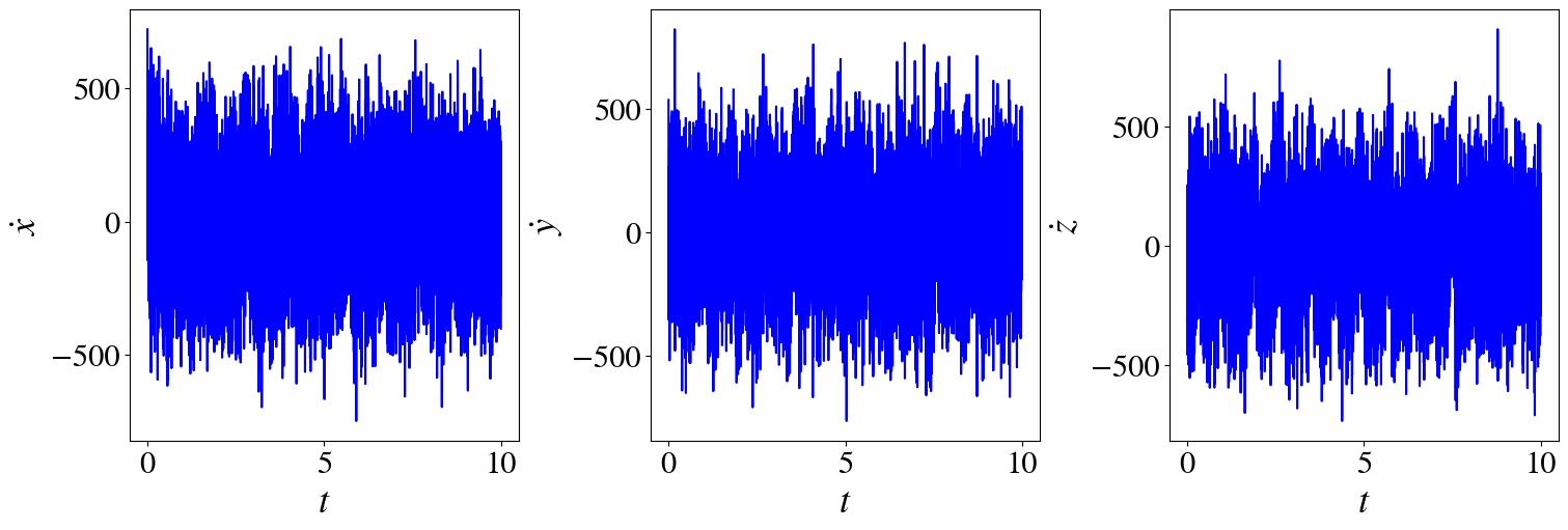
In this exercise, we try to improve the fit of SINDy in the presence of noise. Noise presents a substantial challenge when we are fitting as we have to take the derivative of the data. You can use use a second order library.

Tasks

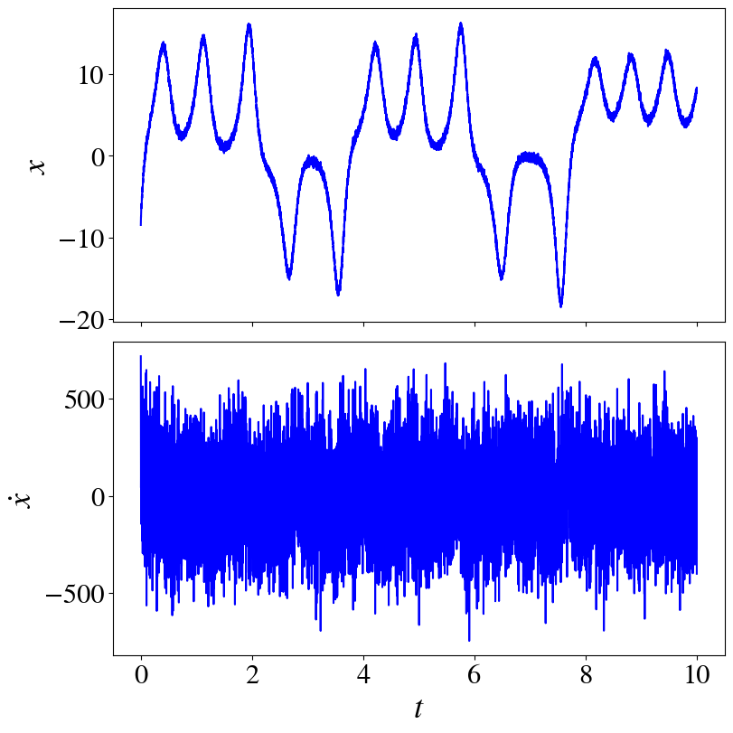
Compare the time series of $x,y,z$ with their derivatives, when $10\%$ noise is added
By using a different method, try to identify a model with $10\%$ noise added.
Now try with $50\%$ noise added. Is it possible to identify a model?

You are also given that the data satisfies the symmetry $x \rightarrow -x, y \rightarrow -y, z \rightarrow z$.

integrator_keywords["args"] = (10, 8/3, 28)
t_train = np.arange(0, 10, dt)
t_train_span = [t_train[0], t_train[-1]]
labels = ["x", "y", "z"]
x_train = solve_ivp(
    lorenz, t_train_span, x0_train, t_eval=t_train, **integrator_keywords
).y.T
#calculate the standard deviation from zero mean
rmse = mean_squared_error(x_train, np.zeros(x_train.shape), squared=False)
#add noise to the measurement data
x_train_noisy = x_train + np.random.normal(0, rmse / 50,  x_train.shape)
xdot_noisy = ps.FiniteDifference()._differentiate(x_train_noisy, t_train)


t_test = np.arange(0, 15, dt)
t_test_span = (t_test[0], t_test[-1])
x0_test = np.array([8, 7, 15])
x_test = solve_ivp(
    lorenz, t_test_span, x0_test, t_eval=t_test, **integrator_keywords
).y.T

fig, axs = plt.subplots(1,3, figsize=(15, 5), layout="constrained")
for i in range(3):
    axs[i].plot(t_train, x_train_noisy[:,i], "b")
    axs[i].set_ylabel(rf"${labels[i]}$")
    axs[i].set_xlabel(
        r"$t$")

fig, axs = plt.subplots(1,3, figsize=(15,5), layout="constrained")
for i in range(3):
    axs[i].plot(t_train, xdot_noisy[:,i], "b")
    axs[i].set_ylabel(r"$\dot}$".format(labels[i]))
    axs[i].set_xlabel(r"$t$")

fig, axs = plt.subplots(2,1, figsize=(8,8), layout="constrained", sharex=True)
axs[0].plot(t_train, x_train_noisy[:,0], "b")
axs[1].plot(t_train, xdot_noisy[:,0], "b")
axs[1].set_xlabel(r"$t$")
axs[0].set_ylabel(r"$x$")
axs[1].set_ylabel(r"$\dot{x}$")

xx=x_train[:,0]
yy=x_train[:,1]
zz=x_train[:,2]

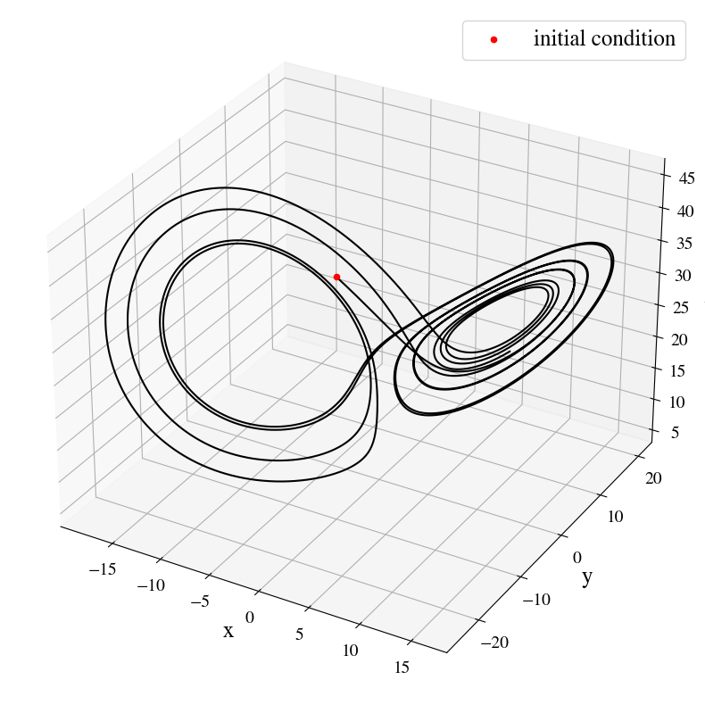
fig = plt.figure(figsize=(10,10))
ax3d = fig.add_subplot(111, projection='3d')
ax3d.plot(xx,yy,zz, "k")
ax3d.scatter(xx[0], yy[0], zz[0], c="r", label="initial condition")
ax3d.set_xlabel(xlabel="x", fontsize=18)
ax3d.set_ylabel(ylabel="y", fontsize=18)
ax3d.set_zlabel(zlabel="z", fontsize=18)
ax3d.tick_params(axis='both', which='major', labelsize=14)
plt.legend(loc="upper right", fontsize=18)#

<matplotlib.legend.Legend at 0x797f06f86d40>

png